For example, consider the logistic map, defined by the simple recurrence formula: \[ x_{n+1} = rx_n(1-x_n) \] For almost all \(r\in[3.567,4]\) this system is chaotic.
A direct encoding in AERN with arbitrary precision support in the style of iRRAM computes tight interval enclosures for \(x_n\). For example, with \(r=3.75\) and \(x_0=0.5\), it computes:
| \(n\) (Number of iterations) | Approx. computation time | Computed enclosure of \(x_n\) |
|---|---|---|
| \(10\) | 0.01 s | \(0.645367290830...\pm 10^{-160}\) |
| \(100\) | 0.02 s | \(0.888293992284...\pm 10^{-160}\) |
| \(1000\) | 0.5 s | \(0.791746740922...\pm 10^{-160}\) |
| \(10,000\) | 64 s | \(0.824204800756...\pm 10^{-160}\) |
| \(100,000\) | 3 h | \(0.666946708411...\pm 10^{-160}\) |
Note that iterating the logistic map is a highly unstable computation. Evaluating it directly using Double precision gives completely meaningless results after not many iterations. For example, for 100 iterations using Double precision one gets \(0.66...\), while the correct number is close to \(0.88...\).
To compute 100,000 iterations with a good precision, the program used floating-point numbers with mantissa size over 200,000 bits. Over 2 hours of the 3-hour computation time was spent trying and failing to perform the computation with various lower precisions.
AERN can bound real continuous functions by function intervals analogously to how it can bound real numbers by real intervals. For example, the demo program erf.hs computes bounds for the error function \[ \begin{equation} \mathrm{erf}(x) =\frac{2}{\sqrt{\pi}}\int_0^x e^{-t^2}\,dt \end{equation} \] over the domain \(x\in[0,2]\). The computed bounds are in the form of an interval \([f(x),g(x)]\) where \(f\) and \(g\) are polynomials such that \(f(x) \leq \mathrm{erf}(x) \leq g(x)\) for all \(x\in[0,2]\). We say that the interval \([f(x),g(x)]\) is an enclosure of the function \(\mathrm{erf}(x)\) over \(x\in[0,2]\).
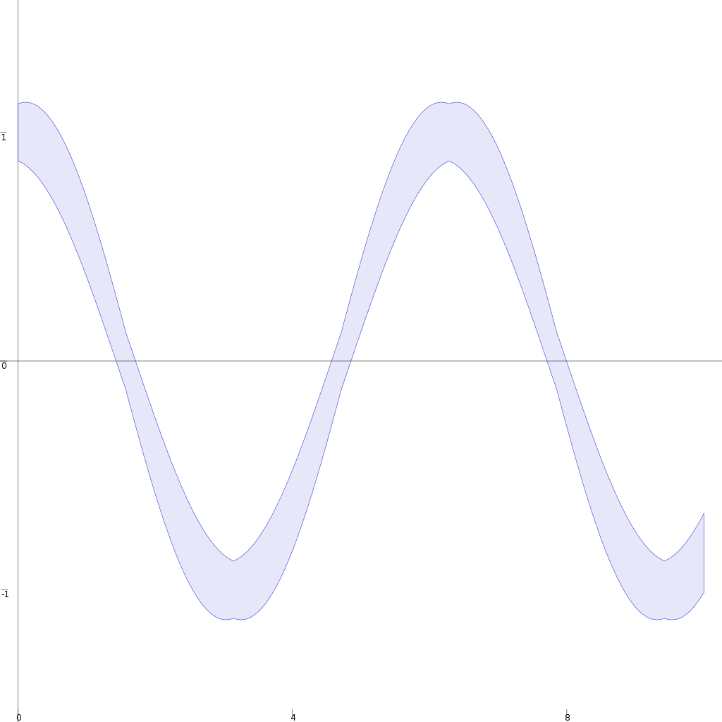
The following plot shows the enclosures for \(\mathrm{erf}(x)\) computed by the program erf.hs:
![Enclosures of the error function over the domain [0,2]](./img/erf-enclosures.png)
Some of the plotted enclosures are rather inaccurate and others are so tight that their thickness is not visible at this zoom level. The quality of the computed enclosure depends on the effort used during the computation. The effort can be set via so-called effort parameters.
For approximating \(\mathrm{erf}(x)\) in AERN there are the following effort parameters:
In our example, all enclosures are computed using the machine Double for polynomial coefficients and interval endpoints, and using the Taylor degree 5.
The upper bound on polynomial degree ranges from 5 to 25.
AERN contains an ODE IVP solver. The main executable of the solver is in the file simple-ode.hs.
First consider the simple harmonic motion initial value problem \[ x'' = -x\qquad x(0) \in 1\pm 0.125\quad x'(0) \in 0\pm 0.125 \] which is formally specified in the module Numeric.AERN.IVP.Examples.ODE.Simple under the name “ivpSpringMass_uv”.
To enclose the solutions of this system, we can run simple-ode as follows:
~/.cabal/bin/simple-ode ivpSpringMass-uv 10 "PlotGraph[True,False](0,10,-1.5,1.5)" GUI ShrinkWrap 30 200 -10 -10producing the following enclosure:
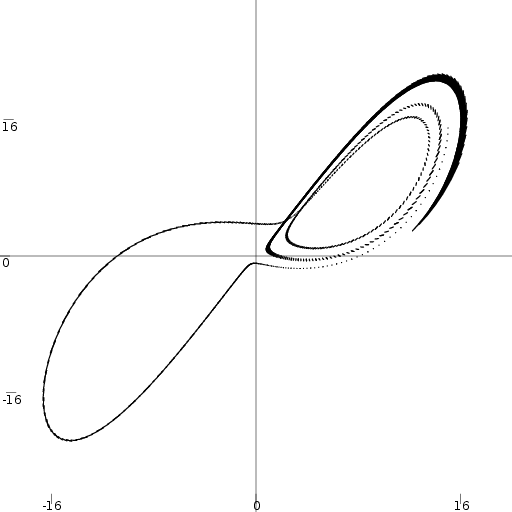
As an example system with chaotic behaviour, consider the classical instance of the Lorenz initial value problem, given by the following ordinary differential equation (ODE) and initial value: \[ \begin{array}{rcl} x' & = & 10(y-x)\\ y' & = & x(28-z)-y\\ z' & = & xy - 8z/3 \end{array} \qquad \begin{array}{rcl} x(0) & \in & 15\pm\delta\\ y(0) & \in & 15\pm\delta\\ z(0) & \in & 36\pm\delta \end{array} \qquad \delta = 0.01 \] which is formally specified in the module Numeric.AERN.IVP.Examples.ODE.Simple under the name “ivpLorenz_uv”.
To enclose the solutions of this system, we can run simple-ode as follows:
~/.cabal/bin/simple-ode ivpLorenz-uv 4 "PlotParam(100,[])[True,True](-20,20,-30,30)" GUI ShrinkWrap 12 200 8 8producing an enclosure whose projection to the \(x\)-\(y\) plane looks as follows:
AERN solve-ode is an experimental solver using an unusual method. It is based on a direct implementation of the interval Picard operator introduced by Edalat & Pattinson (2007). This method of computing solutions is simple, almost correct by construction. Thus one can have a high level of confidence that the solver produces enclosures that contain the exact solution(s). Established enclosure ODE solvers such as VNODE and COSY use more complex methods and are more optimised. The AERN solve-ode solver does not compete with the established solvers in terms of speed and ability to enclose solutions over long time intervals but we expect it will be easier to validate and verify than the established solvers.
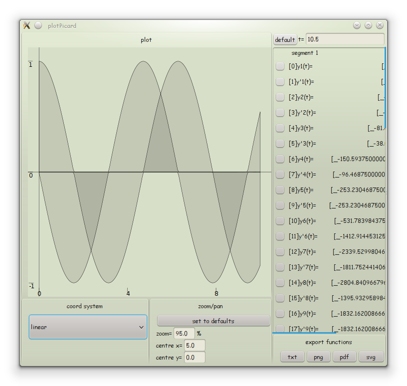
Trajectory of pendulum with an uncertain initial position in a zoomable view widget.